Horizon Distance

The horizon distance, denoted \(D_{\rm hor}\), is a key metric for assessing the sensitivity of a gravitational-wave detector or network. It is defined as the maximum luminosity distance at which a specific GW source can be reliably detected, i.e., where its signal-to-noise ratio (SNR) meets or exceeds a given threshold, typically \(\rho_{\rm th} = 8\).

This distance is computed under the optimal scenario: the source is directly overhead and face-on with respect to the detector(s), providing the strongest possible signal. The gwsnr package offers two approaches for calculating the horizon distance: an analytical scaling method and a numerical root-finding method.

1. Analytical Method

The analytical approach calculates the horizon distance by scaling a known SNR measurement. For any generic inspiral–merger–ringdown (IMR) waveform, the horizon distance can be determined from the optimal SNR (\(\rho_{\rm opt}\)) at a given effective distance (\(D_{\rm eff}\)):

\[ \begin{align} D_{\rm hor} &= \frac{\rho_{\rm opt}}{\rho_{\rm th}} D_{\rm eff}\, \tag{1} \end{align} \]

Notably, this approach does not require explicit optimization over sky location, as the dependence cancels between the SNR and the effective distance.

In gwsnr, \(\rho_{\rm opt}\) is computed using the core functionalities, such as the noise-weighted inner product or the Partial Scaling interpolation method. The package also includes a JIT-compiled function for efficient evaluation of \(D_{\rm eff}\).

This general formula in Eq.(1) is rooted in the work of Allen et al. (2012), which provides a specific analytical expression for simple inspiral waveforms:

\[ \begin{align} D_{\rm hor} &= \left( \frac{1~\mathrm{Mpc}}{\rho_{\rm th}} \right) \mathcal{A}_{1~\mathrm{Mpc}}(\mathcal{M}) \sqrt{ 4 \int_{f_{\rm min}}^{f_{\rm max}} \frac{f^{-7/3}}{S_n(f)}\,df }, \tag{2} \end{align} \]

where \(\mathcal{M}\) is the chirp mass, and \(\mathcal{A}_{1~\mathrm{Mpc}}\) denotes the waveform’s intrinsic amplitude at a distance of 1 Mpc. While Eq.(1) was originally derived for simple inspiral signals, it remains applicable to general IMR waveforms dominated by the quadrupolar (2,2)-mode, provided an appropriate waveform model is used to compute \(\rho_{\rm opt}\).

2. Numerical Method

The numerical method directly determines the horizon distance by finding the specific distance at which the SNR matches the detection threshold. This involves two main steps:

• Optimization: For a given set of relevant GW parameters (masses, spins, phase, etc.), gwsnr first finds the optimal sky location (for each detector) that maximize the SNR, providing the best-case SNR for that source type at a reference distance.

• Root-Finding: With the optimal configuration fixed, the algorithm then numerically solves for the luminosity distance, \(d_L\), that satisfies the equation:

  \[ F(d_L) = \rho(d_L) - \rho_{\rm th} = 0 \]

This approach is also applicable to a network of detectors, in which case the optimal sky location is found for the detector network, where the single-detector SNR, \(\rho\), is replaced by the network SNR, \(\rho_{\rm net}\), and then the root-finding is performed to find the distance at which \(\rho_{\rm net} = \rho_{\rm th}\).

Example Usage

# loading GWSNR class from the gwsnr package
from gwsnr import GWSNR

# initializing the GWSNR class with default configuration and interpolation method
gwsnr = GWSNR(mtot_min=2., mtot_max=6., ifos=['H1', 'L1', 'V1'])

# 1. Analytical Method
d_hor_analytical = gwsnr.horizon_distance_analytical(mass_1=1.4, mass_2=1.4)

# 2. Numerical Method
d_hor_numerical, _, _ = gwsnr.horizon_distance_numerical(mass_1=1.4, mass_2=1.4)

# print the type of the SNRs
print(f"horizon distance (analytical): {d_hor_analytical} Mpc")
print(f"horizon distance (numerical): {d_hor_numerical} Mpc")

horizon distance (analytical): {'L1': array([416.49490771]), 'H1': array([416.49490771]), 'V1': array([317.93916075])} Mpc
horizon distance (numerical): {'L1': 416.49483499582857, 'H1': 416.4948722301051, 'V1': 228.76581222284585, 'snr_net': 557.9508489044383} Mpc

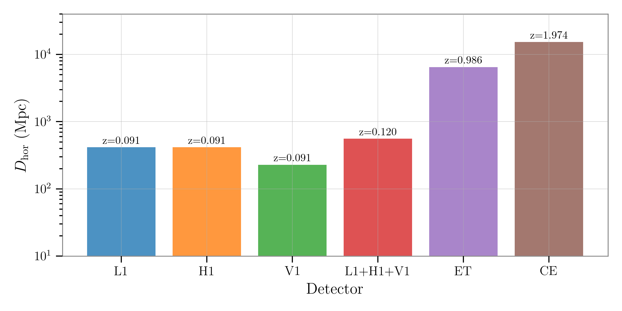
Horizon Distance of a BNS System across various Detectors

Figure. Horizon distance ($D_{\rm hor}$) for binary neutron star (BNS) systems with $m_1=m_2=1.4\,M_\odot$ across various detectors. The bar heights show the maximum detection range (in Mpc, log scale) for the LIGO detectors (L1, H1, V1), their network (L1+H1+V1), and future third-generation observatories (Einstein Telescope, ET; Cosmic Explorer, CE). The annotated values indicate the corresponding redshift at each horizon distance, highlighting the enhanced reach of next-generation detectors.