ANN Model creation and testing

Contents

Training data generation
ANN model training and testing
Implementation of the model in GWSNR

[1]:

# # If you have not installed the following packages, please uncomment and run the following command:
# !pip install ler

1. Training data generation

The training data is generated using ler package.
Data needs to be trained for each detector separately.
I will choose ‘L1’ detector for this notebook with the following specified parameters:
- Sampling frequency : 2048 Hz
- waveform approximant : IMRPhenomXPHM
- minimum frequency : 20.0
- psd : aLIGO_O4_high_asd.txt from pycbc package

[1]:

import numpy as np
import matplotlib.pyplot as plt
from ler.utils import TrainingDataGenerator

[2]:

tdg = TrainingDataGenerator(
    npool=8,  # number of processes
    verbose=False, # set it to True if you are running the code for the first time
    # GWSNR parameters
    sampling_frequency=2048.,
    waveform_approximant='IMRPhenomXPHM',  # spin-precessing waveform model
    minimum_frequency=20.,
    psds={'L1':'aLIGO_O4_high_asd.txt'}, # chosen interferometer is 'L1'. If multiple interferometers are chosen, optimal network SNR will be considered.
    spin_zero=False,
    spin_precessing=True,
    snr_method='inner_product',  # 'interpolation' or 'inner_product'
)

ler package, by default, generates astrophysical signals that most likely will not be detected by the detector, i.e. low SNR signals.
But you want your ANN model to be sensitive to the signals that near the detection threshold.
So, I will generate most of the training data with SNR near the detection threshold.

Note: Increase sample size of the training data to get better accuracy in the ANN model.

[3]:

# rerun if hanged
ler = tdg.gw_parameters_generator(
    size=10000,  # number of samples to generate
    batch_size=400000,  # reduce this number if you have memory issues
    snr_recalculation=True,  # pick SNR generated with 'interpolation'; recalculate SNR using 'inner product'
    trim_to_size=False, verbose=True,
    data_distribution_range = [0., 2., 4., 6., 8., 10., 12., 14., 16., 100.],  # equal data samples will be distributed in these ranges
    replace=False,  # set to True if you want to replace the existing data
    output_jsonfile="IMRPhenomXPHM_O4_high_asd_L1_1.json",
)


Initializing GWRATES class...

current size of the json file: 1197

total event to collect: 10000

100%|████████████████████████████████████████████████████████████| 369/369 [00:00<00:00, 378.22it/s]

Collected number of events: 1485

100%|████████████████████████████████████████████████████████████| 378/378 [00:00<00:00, 398.39it/s]

Collected number of events: 1773

100%|████████████████████████████████████████████████████████████| 314/314 [00:00<00:00, 354.46it/s]

Collected number of events: 2043

100%|████████████████████████████████████████████████████████████| 423/423 [00:01<00:00, 399.50it/s]

Collected number of events: 2412

100%|████████████████████████████████████████████████████████████| 338/338 [00:00<00:00, 362.23it/s]

Collected number of events: 2691

100%|████████████████████████████████████████████████████████████| 454/454 [00:01<00:00, 409.53it/s]

Collected number of events: 3006

100%|████████████████████████████████████████████████████████████| 449/449 [00:01<00:00, 400.76it/s]

Collected number of events: 3348

100%|████████████████████████████████████████████████████████████| 279/279 [00:00<00:00, 348.12it/s]

Collected number of events: 3582

100%|████████████████████████████████████████████████████████████| 396/396 [00:01<00:00, 374.89it/s]

Collected number of events: 3915

100%|████████████████████████████████████████████████████████████| 387/387 [00:00<00:00, 402.89it/s]

Collected number of events: 4257

100%|████████████████████████████████████████████████████████████| 395/395 [00:01<00:00, 383.34it/s]

Collected number of events: 4545

100%|████████████████████████████████████████████████████████████| 377/377 [00:01<00:00, 366.50it/s]

Collected number of events: 4833

100%|████████████████████████████████████████████████████████████| 377/377 [00:00<00:00, 389.85it/s]

Collected number of events: 5166

100%|████████████████████████████████████████████████████████████| 396/396 [00:01<00:00, 389.59it/s]

Collected number of events: 5472

100%|████████████████████████████████████████████████████████████| 405/405 [00:01<00:00, 378.78it/s]

Collected number of events: 5769

100%|████████████████████████████████████████████████████████████| 387/387 [00:01<00:00, 382.65it/s]

Collected number of events: 6138

100%|████████████████████████████████████████████████████████████| 259/259 [00:00<00:00, 339.38it/s]

Collected number of events: 6336

100%|████████████████████████████████████████████████████████████| 315/315 [00:00<00:00, 353.23it/s]

Collected number of events: 6588

100%|████████████████████████████████████████████████████████████| 378/378 [00:01<00:00, 363.57it/s]

Collected number of events: 6849

100%|████████████████████████████████████████████████████████████| 297/297 [00:00<00:00, 342.76it/s]

Collected number of events: 7092

100%|████████████████████████████████████████████████████████████| 305/305 [00:00<00:00, 361.80it/s]

Collected number of events: 7317

100%|████████████████████████████████████████████████████████████| 332/332 [00:00<00:00, 376.09it/s]

Collected number of events: 7560

100%|████████████████████████████████████████████████████████████| 377/377 [00:00<00:00, 388.24it/s]

Collected number of events: 7875

100%|████████████████████████████████████████████████████████████| 306/306 [00:00<00:00, 348.02it/s]

Collected number of events: 8127

100%|████████████████████████████████████████████████████████████| 421/421 [00:01<00:00, 394.64it/s]

Collected number of events: 8424

100%|████████████████████████████████████████████████████████████| 377/377 [00:01<00:00, 371.58it/s]

Collected number of events: 8775

100%|████████████████████████████████████████████████████████████| 432/432 [00:01<00:00, 393.02it/s]

Collected number of events: 9144

100%|████████████████████████████████████████████████████████████| 304/304 [00:00<00:00, 334.92it/s]

Collected number of events: 9396

100%|████████████████████████████████████████████████████████████| 466/466 [00:01<00:00, 438.22it/s]

Collected number of events: 9765

100%|████████████████████████████████████████████████████████████| 369/369 [00:00<00:00, 390.73it/s]

Collected number of events: 10098
final size: 10098

json file saved at: ./ler_data/IMRPhenomXPHM_O4_high_asd_L1_1.json

[ ]:

[4]:

# might take 2mins~3mins
# 10 mins 0.7 s, 10000 samples with 8 processes and batch_size=200000
tdg.gw_parameters_generator(
    size=5000,
    batch_size=200000,
    snr_recalculation=True,
    trim_to_size=False, verbose=True,
    data_distribution_range = [4., 8., 12.], # equal data samples will be distributed in these ranges
    replace=False,
    output_jsonfile="IMRPhenomXPHM_O4_high_asd_L1_2.json",
)


Initializing GWRATES class...

total event to collect: 5000

100%|████████████████████████████████████████████████████████████| 438/438 [00:01<00:00, 426.01it/s]

Collected number of events: 376

100%|████████████████████████████████████████████████████████████| 494/494 [00:01<00:00, 444.68it/s]

Collected number of events: 816

100%|████████████████████████████████████████████████████████████| 480/480 [00:01<00:00, 417.20it/s]

Collected number of events: 1224

100%|████████████████████████████████████████████████████████████| 464/464 [00:01<00:00, 409.93it/s]

Collected number of events: 1630

100%|████████████████████████████████████████████████████████████| 482/482 [00:01<00:00, 392.78it/s]

Collected number of events: 2060

100%|████████████████████████████████████████████████████████████| 470/470 [00:01<00:00, 387.19it/s]

Collected number of events: 2460

100%|████████████████████████████████████████████████████████████| 472/472 [00:01<00:00, 412.21it/s]

Collected number of events: 2856

100%|████████████████████████████████████████████████████████████| 470/470 [00:01<00:00, 423.07it/s]

Collected number of events: 3272

100%|████████████████████████████████████████████████████████████| 530/530 [00:01<00:00, 430.88it/s]

Collected number of events: 3712

100%|████████████████████████████████████████████████████████████| 438/438 [00:01<00:00, 405.48it/s]

Collected number of events: 4092

100%|████████████████████████████████████████████████████████████| 486/486 [00:01<00:00, 419.60it/s]

Collected number of events: 4516

100%|████████████████████████████████████████████████████████████| 466/466 [00:01<00:00, 379.73it/s]

Collected number of events: 4922

100%|████████████████████████████████████████████████████████████| 498/498 [00:01<00:00, 441.36it/s]

Collected number of events: 5362
final size: 5362

json file saved at: ./ler_data/IMRPhenomXPHM_O4_high_asd_L1_2.json

[5]:

tdg.gw_parameters_generator(
    size=10000,
    batch_size=10000,
    snr_recalculation=True,
    trim_to_size=False,
    verbose=False,
    data_distribution_range = None,
    replace=True,
    output_jsonfile="IMRPhenomXPHM_O4_high_asd_L1_3.json",
)


Initializing GWRATES class...

total event to collect: 10000

final size: 10000

json file saved at: ./ler_data/IMRPhenomXPHM_O4_high_asd_L1_3.json

Additional random samples

[6]:

from gwsnr import GWSNR
import numpy as np

gwsnr = GWSNR(
    npool=8,  # number of processes
    # GWSNR parameters
    sampling_frequency=2048.,
    waveform_approximant='IMRPhenomXPHM',  # spin-precessing waveform model
    minimum_frequency=20.,
    psds={'L1':'aLIGO_O4_high_asd.txt'}, # chosen interferometer is 'L1'. If multiple network SNR will be considered.
    snr_method='inner_product',  # 'interpolation' or 'inner_product'
)


Initializing GWSNR class...

Intel processor has trouble allocating memory when the data is huge. So, by default for IMRPhenomXPHM, duration_max = 64.0. Otherwise, set to some max value like duration_max = 600.0 (10 mins)

Chosen GWSNR initialization parameters:

npool:  8
snr type:  inner_product
waveform approximant:  IMRPhenomXPHM
sampling frequency:  2048.0
minimum frequency (fmin):  20.0
mtot=mass1+mass2
min(mtot):  9.96
max(mtot) (with the given fmin=20.0): 235.0
detectors:  ['L1']
psds:  [PowerSpectralDensity(psd_file='None', asd_file='/Users/phurailatpamhemantakumar/anaconda3/envs/ler/lib/python3.10/site-packages/bilby/gw/detector/noise_curves/aLIGO_O4_high_asd.txt')]

[7]:

# gerneral case, random parameters
np.random.seed(64)
nsamples = 50000
mtot = np.random.uniform(2*4.98, 2*112.5,nsamples)
mass_ratio = np.random.uniform(0.2,1,size=nsamples)
param_dict = dict(
    # convert to component masses
    mass_1 = mtot / (1 + mass_ratio),
    mass_2 = mtot * mass_ratio / (1 + mass_ratio),
    # Fix luminosity distance
    luminosity_distance = np.random.uniform(40, 10000, size=nsamples),  # Random luminosity distance between 40 and 10000 Mpc
    # Randomly sample everything else:
    theta_jn = np.random.uniform(0,2*np.pi, size=nsamples),
    ra = np.random.uniform(0,2*np.pi, size=nsamples),
    dec = np.random.uniform(-np.pi/2,np.pi/2, size=nsamples),
    psi = np.random.uniform(0,2*np.pi, size=nsamples),
    phase = np.random.uniform(0,2*np.pi, size=nsamples),
    geocent_time = 1246527224.169434*np.ones(nsamples),
    # spin zero
    a_1 = np.random.uniform(0.0,0.8, size=nsamples),
    a_2 = np.random.uniform(0.0,0.8, size=nsamples),
    tilt_1 = np.random.uniform(0, np.pi, size=nsamples),  # tilt angle of the primary black hole in radians
    tilt_2 = np.random.uniform(0, np.pi, size=nsamples),
    phi_12 = np.random.uniform(0, 2*np.pi, size=nsamples),  # Relative angle between the primary and secondary spin of the binary in radians
    phi_jl = np.random.uniform(0, 2*np.pi, size=nsamples),  # Angle between the total angular momentum and the orbital angular momentum in radians
)

snrs_ = gwsnr.optimal_snr(gw_param_dict=param_dict)
# time: 0.2 s for 50000 samples with 8 processes

solving SNR with inner product

100%|███████████████████████████████████████████████████████| 50000/50000 [00:40<00:00, 1247.30it/s]

[8]:

param_dict.update(snrs_)
from gwsnr.utils import append_json
append_json(
    file_name="ler_data/IMRPhenomXPHM_O4_high_asd_L1_4.json",
    new_dictionary =param_dict,
    replace=True,  # set to True if you want to replace the existing data
);

[ ]:

Combine all the data files into one

L1 detector

[9]:

import numpy as np
import matplotlib.pyplot as plt
from ler.utils import TrainingDataGenerator

tdg = TrainingDataGenerator()
tdg.combine_dicts(
    file_name_list=["IMRPhenomXPHM_O4_high_asd_L1_1.json", "IMRPhenomXPHM_O4_high_asd_L1_2.json", "IMRPhenomXPHM_O4_high_asd_L1_3.json", "IMRPhenomXPHM_O4_high_asd_L1_4.json"],
    detector='L1',
    output_jsonfile="IMRPhenomXPHM_O4_high_asd_L1.json",
)

json file saved at: ./ler_data/IMRPhenomXPHM_O4_high_asd_L1.json

[10]:

# from gwsnr.utils import get_param_from_json
# test1 = get_param_from_json("./ler_data/IMRPhenomXPHM_O4_high_asd_L1.json")

# snr = np.array(test1['L1'])
# print(f"Number of samples: {len(snr)}")

# plt.figure(figsize=[4,4])
# plt.hist(snr, bins=100, density=True, alpha=0.5, color='b', histtype='step', label='L1')
# plt.xlim([0, 40])
# plt.xlabel('Optimal SNR')
# plt.ylabel('Density')
# plt.legend()
# plt.show()

ANN model training and testing

[11]:

import numpy as np
import matplotlib.pyplot as plt
from gwsnr.ann import ANNModelGenerator

[12]:

amg = ANNModelGenerator(
    directory='./ann_data',
    npool=8,
    gwsnr_verbose=False,
    snr_th=8.0,
    waveform_approximant="IMRPhenomXPHM",
    psds={'L1': 'aLIGO_O4_high_asd.txt'},
)


Initializing GWSNR class...

Intel processor has trouble allocating memory when the data is huge. So, by default for IMRPhenomXPHM, duration_max = 64.0. Otherwise, set to some max value like duration_max = 600.0 (10 mins)
Interpolator will be loaded for L1 detector from ./interpolator_pickle/L1/partialSNR_dict_1.pickle

[13]:

amg.ann_model_training(
    gw_param_dict='ler_data/IMRPhenomXPHM_O4_high_asd_L1.json', # you can also get the dict from a json file first
    randomize=True,
    test_size=0.1,
    random_state=42,
    num_nodes_list = [5, 32, 32, 1],
    activation_fn_list = ['relu', 'relu', 'sigmoid', 'linear'],
    optimizer='adam',
    loss='mean_squared_error',
    metrics=['accuracy'],
    batch_size=32,
    epochs=100,
    error_adjustment_snr_range=[2,14],
    ann_file_name = 'ann_model_L1.h5',
    scaler_file_name = 'scaler_L1.pkl',
    error_adjustment_file_name='error_adjustment_L1.json',
    ann_path_dict_file_name='ann_path_dict.json',
)

# # Uncomment the following, if you have already trained the model
# # load the trained model
# amg.load_model_scaler_error(
#     ann_file_name='ann_model_L1.h5',
#     scaler_file_name='scaler_L1.pkl',
#     error_adjustment_file_name='error_adjustment_L1.json',
# )

Epoch 1/100
2123/2123 ━━━━━━━━━━━━━━━━━━━━ 1s 309us/step - accuracy: 7.4186e-04 - loss: 1195.4056
Epoch 2/100
2123/2123 ━━━━━━━━━━━━━━━━━━━━ 1s 303us/step - accuracy: 3.7843e-04 - loss: 786.9496
Epoch 3/100
2123/2123 ━━━━━━━━━━━━━━━━━━━━ 1s 338us/step - accuracy: 5.5559e-04 - loss: 773.3979
Epoch 4/100
2123/2123 ━━━━━━━━━━━━━━━━━━━━ 1s 312us/step - accuracy: 4.7510e-04 - loss: 870.4972
Epoch 5/100
2123/2123 ━━━━━━━━━━━━━━━━━━━━ 1s 302us/step - accuracy: 5.0608e-04 - loss: 669.6340
Epoch 6/100
2123/2123 ━━━━━━━━━━━━━━━━━━━━ 1s 340us/step - accuracy: 2.4172e-04 - loss: 599.0781
Epoch 7/100
2123/2123 ━━━━━━━━━━━━━━━━━━━━ 1s 296us/step - accuracy: 1.1708e-04 - loss: 615.2960
Epoch 8/100
2123/2123 ━━━━━━━━━━━━━━━━━━━━ 1s 296us/step - accuracy: 4.0820e-04 - loss: 504.8292
Epoch 9/100
2123/2123 ━━━━━━━━━━━━━━━━━━━━ 1s 325us/step - accuracy: 3.1350e-04 - loss: 473.1070
Epoch 10/100
2123/2123 ━━━━━━━━━━━━━━━━━━━━ 1s 318us/step - accuracy: 4.6338e-04 - loss: 455.0616
Epoch 11/100
2123/2123 ━━━━━━━━━━━━━━━━━━━━ 1s 313us/step - accuracy: 3.6646e-04 - loss: 480.0711
Epoch 12/100
2123/2123 ━━━━━━━━━━━━━━━━━━━━ 1s 331us/step - accuracy: 6.4646e-04 - loss: 430.3829
Epoch 13/100
2123/2123 ━━━━━━━━━━━━━━━━━━━━ 1s 331us/step - accuracy: 4.6718e-04 - loss: 326.0745
Epoch 14/100
2123/2123 ━━━━━━━━━━━━━━━━━━━━ 1s 321us/step - accuracy: 4.8356e-04 - loss: 344.0058
Epoch 15/100
2123/2123 ━━━━━━━━━━━━━━━━━━━━ 1s 333us/step - accuracy: 6.9886e-04 - loss: 318.9627
Epoch 16/100
2123/2123 ━━━━━━━━━━━━━━━━━━━━ 1s 360us/step - accuracy: 6.3820e-04 - loss: 316.1301
Epoch 17/100
2123/2123 ━━━━━━━━━━━━━━━━━━━━ 1s 327us/step - accuracy: 6.0792e-04 - loss: 301.1277
Epoch 18/100
2123/2123 ━━━━━━━━━━━━━━━━━━━━ 1s 315us/step - accuracy: 6.6761e-04 - loss: 235.1516
Epoch 19/100
2123/2123 ━━━━━━━━━━━━━━━━━━━━ 1s 315us/step - accuracy: 6.2474e-04 - loss: 272.7290
Epoch 20/100
2123/2123 ━━━━━━━━━━━━━━━━━━━━ 1s 314us/step - accuracy: 7.3992e-04 - loss: 290.7437
Epoch 21/100
2123/2123 ━━━━━━━━━━━━━━━━━━━━ 1s 312us/step - accuracy: 4.9990e-04 - loss: 207.5985
Epoch 22/100
2123/2123 ━━━━━━━━━━━━━━━━━━━━ 1s 319us/step - accuracy: 8.0967e-04 - loss: 263.7404
Epoch 23/100
2123/2123 ━━━━━━━━━━━━━━━━━━━━ 1s 312us/step - accuracy: 7.1809e-04 - loss: 235.5507
Epoch 24/100
2123/2123 ━━━━━━━━━━━━━━━━━━━━ 1s 309us/step - accuracy: 6.9704e-04 - loss: 171.0875
Epoch 25/100
2123/2123 ━━━━━━━━━━━━━━━━━━━━ 1s 314us/step - accuracy: 9.5122e-04 - loss: 188.7950
Epoch 26/100
2123/2123 ━━━━━━━━━━━━━━━━━━━━ 1s 318us/step - accuracy: 9.8965e-04 - loss: 200.5005
Epoch 27/100
2123/2123 ━━━━━━━━━━━━━━━━━━━━ 1s 312us/step - accuracy: 7.1190e-04 - loss: 219.7502
Epoch 28/100
2123/2123 ━━━━━━━━━━━━━━━━━━━━ 1s 311us/step - accuracy: 8.6508e-04 - loss: 195.2021
Epoch 29/100
2123/2123 ━━━━━━━━━━━━━━━━━━━━ 1s 313us/step - accuracy: 0.0010 - loss: 162.9744
Epoch 30/100
2123/2123 ━━━━━━━━━━━━━━━━━━━━ 1s 316us/step - accuracy: 8.3644e-04 - loss: 163.9187
Epoch 31/100
2123/2123 ━━━━━━━━━━━━━━━━━━━━ 1s 322us/step - accuracy: 9.6832e-04 - loss: 186.6651
Epoch 32/100
2123/2123 ━━━━━━━━━━━━━━━━━━━━ 1s 350us/step - accuracy: 0.0010 - loss: 160.6446
Epoch 33/100
2123/2123 ━━━━━━━━━━━━━━━━━━━━ 1s 318us/step - accuracy: 0.0011 - loss: 110.9650
Epoch 34/100
2123/2123 ━━━━━━━━━━━━━━━━━━━━ 1s 316us/step - accuracy: 0.0011 - loss: 148.0654
Epoch 35/100
2123/2123 ━━━━━━━━━━━━━━━━━━━━ 1s 320us/step - accuracy: 0.0013 - loss: 118.0238
Epoch 36/100
2123/2123 ━━━━━━━━━━━━━━━━━━━━ 1s 330us/step - accuracy: 0.0014 - loss: 119.6208
Epoch 37/100
2123/2123 ━━━━━━━━━━━━━━━━━━━━ 1s 315us/step - accuracy: 0.0013 - loss: 123.7099
Epoch 38/100
2123/2123 ━━━━━━━━━━━━━━━━━━━━ 1s 311us/step - accuracy: 0.0014 - loss: 150.7826
Epoch 39/100
2123/2123 ━━━━━━━━━━━━━━━━━━━━ 1s 311us/step - accuracy: 0.0014 - loss: 132.0962
Epoch 40/100
2123/2123 ━━━━━━━━━━━━━━━━━━━━ 1s 311us/step - accuracy: 0.0015 - loss: 112.5593
Epoch 41/100
2123/2123 ━━━━━━━━━━━━━━━━━━━━ 1s 326us/step - accuracy: 0.0012 - loss: 108.4442
Epoch 42/100
2123/2123 ━━━━━━━━━━━━━━━━━━━━ 1s 318us/step - accuracy: 0.0015 - loss: 131.0688
Epoch 43/100
2123/2123 ━━━━━━━━━━━━━━━━━━━━ 1s 311us/step - accuracy: 0.0015 - loss: 130.2682
Epoch 44/100
2123/2123 ━━━━━━━━━━━━━━━━━━━━ 1s 310us/step - accuracy: 0.0018 - loss: 92.5214
Epoch 45/100
2123/2123 ━━━━━━━━━━━━━━━━━━━━ 1s 312us/step - accuracy: 0.0015 - loss: 118.0394
Epoch 46/100
2123/2123 ━━━━━━━━━━━━━━━━━━━━ 1s 321us/step - accuracy: 0.0017 - loss: 87.9507
Epoch 47/100
2123/2123 ━━━━━━━━━━━━━━━━━━━━ 1s 313us/step - accuracy: 0.0016 - loss: 83.3415
Epoch 48/100
2123/2123 ━━━━━━━━━━━━━━━━━━━━ 1s 346us/step - accuracy: 0.0014 - loss: 114.2209
Epoch 49/100
2123/2123 ━━━━━━━━━━━━━━━━━━━━ 1s 313us/step - accuracy: 0.0016 - loss: 56.4827
Epoch 50/100
2123/2123 ━━━━━━━━━━━━━━━━━━━━ 1s 313us/step - accuracy: 0.0015 - loss: 73.1249
Epoch 51/100
2123/2123 ━━━━━━━━━━━━━━━━━━━━ 1s 320us/step - accuracy: 0.0015 - loss: 64.7108
Epoch 52/100
2123/2123 ━━━━━━━━━━━━━━━━━━━━ 1s 311us/step - accuracy: 0.0016 - loss: 80.9203
Epoch 53/100
2123/2123 ━━━━━━━━━━━━━━━━━━━━ 1s 312us/step - accuracy: 0.0018 - loss: 73.7451
Epoch 54/100
2123/2123 ━━━━━━━━━━━━━━━━━━━━ 1s 310us/step - accuracy: 0.0012 - loss: 81.1201
Epoch 55/100
2123/2123 ━━━━━━━━━━━━━━━━━━━━ 1s 322us/step - accuracy: 0.0017 - loss: 79.5091
Epoch 56/100
2123/2123 ━━━━━━━━━━━━━━━━━━━━ 1s 313us/step - accuracy: 0.0015 - loss: 49.4225
Epoch 57/100
2123/2123 ━━━━━━━━━━━━━━━━━━━━ 1s 315us/step - accuracy: 0.0018 - loss: 74.7164
Epoch 58/100
2123/2123 ━━━━━━━━━━━━━━━━━━━━ 1s 312us/step - accuracy: 0.0019 - loss: 70.6322
Epoch 59/100
2123/2123 ━━━━━━━━━━━━━━━━━━━━ 1s 312us/step - accuracy: 0.0017 - loss: 56.8413
Epoch 60/100
2123/2123 ━━━━━━━━━━━━━━━━━━━━ 1s 325us/step - accuracy: 0.0018 - loss: 56.4192
Epoch 61/100
2123/2123 ━━━━━━━━━━━━━━━━━━━━ 1s 319us/step - accuracy: 0.0015 - loss: 45.2987
Epoch 62/100
2123/2123 ━━━━━━━━━━━━━━━━━━━━ 1s 342us/step - accuracy: 0.0017 - loss: 69.9411
Epoch 63/100
2123/2123 ━━━━━━━━━━━━━━━━━━━━ 1s 316us/step - accuracy: 0.0017 - loss: 79.2437
Epoch 64/100
2123/2123 ━━━━━━━━━━━━━━━━━━━━ 1s 324us/step - accuracy: 0.0015 - loss: 65.2600
Epoch 65/100
2123/2123 ━━━━━━━━━━━━━━━━━━━━ 1s 313us/step - accuracy: 0.0018 - loss: 82.6208
Epoch 66/100
2123/2123 ━━━━━━━━━━━━━━━━━━━━ 1s 311us/step - accuracy: 0.0019 - loss: 33.4129
Epoch 67/100
2123/2123 ━━━━━━━━━━━━━━━━━━━━ 1s 309us/step - accuracy: 0.0014 - loss: 51.1544
Epoch 68/100
2123/2123 ━━━━━━━━━━━━━━━━━━━━ 1s 311us/step - accuracy: 0.0015 - loss: 41.7268
Epoch 69/100
2123/2123 ━━━━━━━━━━━━━━━━━━━━ 1s 319us/step - accuracy: 0.0015 - loss: 47.2896
Epoch 70/100
2123/2123 ━━━━━━━━━━━━━━━━━━━━ 1s 351us/step - accuracy: 0.0015 - loss: 53.9465
Epoch 71/100
2123/2123 ━━━━━━━━━━━━━━━━━━━━ 1s 314us/step - accuracy: 0.0020 - loss: 55.2872
Epoch 72/100
2123/2123 ━━━━━━━━━━━━━━━━━━━━ 1s 310us/step - accuracy: 0.0014 - loss: 37.5868
Epoch 73/100
2123/2123 ━━━━━━━━━━━━━━━━━━━━ 1s 314us/step - accuracy: 0.0016 - loss: 48.0865
Epoch 74/100
2123/2123 ━━━━━━━━━━━━━━━━━━━━ 1s 321us/step - accuracy: 0.0018 - loss: 59.0398
Epoch 75/100
2123/2123 ━━━━━━━━━━━━━━━━━━━━ 1s 313us/step - accuracy: 0.0014 - loss: 80.2237
Epoch 76/100
2123/2123 ━━━━━━━━━━━━━━━━━━━━ 1s 312us/step - accuracy: 0.0016 - loss: 43.6412
Epoch 77/100
2123/2123 ━━━━━━━━━━━━━━━━━━━━ 1s 312us/step - accuracy: 0.0015 - loss: 40.7872
Epoch 78/100
2123/2123 ━━━━━━━━━━━━━━━━━━━━ 1s 310us/step - accuracy: 0.0014 - loss: 40.5094
Epoch 79/100
2123/2123 ━━━━━━━━━━━━━━━━━━━━ 1s 318us/step - accuracy: 0.0016 - loss: 53.2459
Epoch 80/100
2123/2123 ━━━━━━━━━━━━━━━━━━━━ 1s 315us/step - accuracy: 0.0019 - loss: 46.4946
Epoch 81/100
2123/2123 ━━━━━━━━━━━━━━━━━━━━ 1s 313us/step - accuracy: 0.0018 - loss: 39.9218
Epoch 82/100
2123/2123 ━━━━━━━━━━━━━━━━━━━━ 1s 318us/step - accuracy: 0.0017 - loss: 35.7595
Epoch 83/100
2123/2123 ━━━━━━━━━━━━━━━━━━━━ 1s 326us/step - accuracy: 0.0017 - loss: 36.7095
Epoch 84/100
2123/2123 ━━━━━━━━━━━━━━━━━━━━ 1s 371us/step - accuracy: 0.0020 - loss: 30.4304
Epoch 85/100
2123/2123 ━━━━━━━━━━━━━━━━━━━━ 1s 320us/step - accuracy: 0.0021 - loss: 34.6025
Epoch 86/100
2123/2123 ━━━━━━━━━━━━━━━━━━━━ 1s 332us/step - accuracy: 0.0020 - loss: 33.1985
Epoch 87/100
2123/2123 ━━━━━━━━━━━━━━━━━━━━ 1s 333us/step - accuracy: 0.0020 - loss: 25.5399
Epoch 88/100
2123/2123 ━━━━━━━━━━━━━━━━━━━━ 1s 352us/step - accuracy: 0.0016 - loss: 40.3483
Epoch 89/100
2123/2123 ━━━━━━━━━━━━━━━━━━━━ 1s 322us/step - accuracy: 0.0016 - loss: 38.8713
Epoch 90/100
2123/2123 ━━━━━━━━━━━━━━━━━━━━ 1s 312us/step - accuracy: 0.0016 - loss: 36.6795
Epoch 91/100
2123/2123 ━━━━━━━━━━━━━━━━━━━━ 1s 314us/step - accuracy: 0.0015 - loss: 35.2267
Epoch 92/100
2123/2123 ━━━━━━━━━━━━━━━━━━━━ 1s 316us/step - accuracy: 0.0018 - loss: 26.4520
Epoch 93/100
2123/2123 ━━━━━━━━━━━━━━━━━━━━ 1s 313us/step - accuracy: 0.0016 - loss: 27.2608
Epoch 94/100
2123/2123 ━━━━━━━━━━━━━━━━━━━━ 1s 329us/step - accuracy: 0.0017 - loss: 33.0001
Epoch 95/100
2123/2123 ━━━━━━━━━━━━━━━━━━━━ 1s 313us/step - accuracy: 0.0019 - loss: 33.2583
Epoch 96/100
2123/2123 ━━━━━━━━━━━━━━━━━━━━ 1s 316us/step - accuracy: 0.0017 - loss: 28.9015
Epoch 97/100
2123/2123 ━━━━━━━━━━━━━━━━━━━━ 1s 328us/step - accuracy: 0.0019 - loss: 24.7544
Epoch 98/100
2123/2123 ━━━━━━━━━━━━━━━━━━━━ 1s 331us/step - accuracy: 0.0018 - loss: 27.0456
Epoch 99/100
2123/2123 ━━━━━━━━━━━━━━━━━━━━ 1s 316us/step - accuracy: 0.0018 - loss: 27.1680
Epoch 100/100
2123/2123 ━━━━━━━━━━━━━━━━━━━━ 1s 351us/step - accuracy: 0.0014 - loss: 33.9702
236/236 ━━━━━━━━━━━━━━━━━━━━ 0s 297us/step
scaler saved at: ./ann_data/scaler_L1.pkl
model saved at: ./ann_data/ann_model_L1.h5
error adjustment saved at: ./ann_data/error_adjustment_L1.json
ann path dict saved at: ./ann_data/ann_path_dict.json

[14]:

amg.pdet_error()

236/236 ━━━━━━━━━━━━━━━━━━━━ 0s 242us/step
Error: 3.45%

[14]:

(3.445534057778956,
 array([14.857255 ,  0.5539622,  2.7361565, ..., 12.17969  ,
        30.18567  , 30.088642 ], dtype=float32),
 array([14.48240752,  0.67263087,  3.5234792 , ..., 12.18434598,
        30.22166581, 30.23929325]))

[15]:

amg.pdet_confusion_matrix()

236/236 ━━━━━━━━━━━━━━━━━━━━ 0s 243us/step
[[5338   85]
 [ 195 1928]]
Accuracy: 96.289%

[15]:

(array([[5338,   85],
        [ 195, 1928]]),
 96.28942486085343,
 array([ True, False, False, ...,  True,  True,  True]),
 array([ True, False, False, ...,  True,  True,  True]))

[16]:

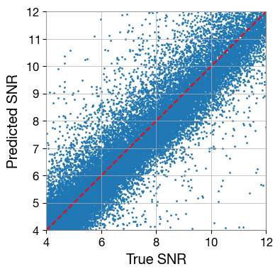
# predicted snr
pred_snr= amg.predict_snr(gw_param_dict='ler_data/IMRPhenomXPHM_O4_high_asd_L1.json')
# true snr
true_snr = amg.get_parameters(gw_param_dict='ler_data/IMRPhenomXPHM_O4_high_asd_L1.json')['L1']
# select only snr between 4 and 12
snr_min = 4
snr_max = 12
mask = (true_snr >= snr_min) & (true_snr <= snr_max)
true_snr = true_snr[mask]
pred_snr = pred_snr[mask]

# plot the predicted snr vs true snr
plt.figure(figsize=[4,4])
plt.scatter(true_snr, pred_snr, s=1)
snr_lim = [np.min([true_snr, true_snr]), np.max([true_snr, true_snr])]
plt.plot(snr_lim, snr_lim, 'r--')
plt.xlabel('True SNR')
plt.ylabel('Predicted SNR')
plt.xlim([snr_min, snr_max])
plt.ylim([snr_min, snr_max])
plt.show()

2359/2359 ━━━━━━━━━━━━━━━━━━━━ 1s 213us/step

../_images/examples_model_generation_25_1.png

[17]:

# use the following function to predict the pdet
pred_pdet = amg.predict_pdet(gw_param_dict='ler_data/IMRPhenomXPHM_O4_high_asd_L1.json', snr_threshold=8.0)

true_snr = amg.get_parameters(gw_param_dict='ler_data/IMRPhenomXPHM_O4_high_asd_L1.json')['L1']
# true pdet
true_pdet = np.array([1 if snr >= 8.0 else 0 for snr in true_snr])

from sklearn.metrics import confusion_matrix, accuracy_score
cm = confusion_matrix(true_pdet, pred_pdet)
print(cm)

acc = accuracy_score(true_pdet, pred_pdet)
print(acc)

2359/2359 ━━━━━━━━━━━━━━━━━━━━ 1s 222us/step
[[53130   947]
 [ 1464 19919]]
0.9680492976411343

[ ]:

3. Implementation of the ANN model in GWSNR

Generate new astrophysical data and test the model on it using GWSNR class.

[18]:

from ler.utils import TrainingDataGenerator

# generate some new data
tdg = TrainingDataGenerator(
    npool=4,
    verbose=False,
    # GWSNR parameters
    sampling_frequency=2048,
    waveform_approximant='IMRPhenomXPHM',
    psds={'L1': 'aLIGO_O4_high_asd.txt'},
    minimum_frequency=20,
    spin_zero=False,
    spin_precessing=True,
    snr_method='inner_product',
)

tdg.gw_parameters_generator(
    size=20000,
    batch_size=20000,
    snr_recalculation=False,
    trim_to_size=False,
    verbose=True,
    data_distribution_range = None,
    replace=False,
    output_jsonfile="IMRPhenomXPHM_O4_high_asd_L1_5.json",
)


Initializing GWRATES class...

total event to collect: 20000

100%|████████████████████████████████████████████████████████| 19507/19507 [00:26<00:00, 724.89it/s]

Collected number of events: 20000
final size: 20000

json file saved at: ./ler_data/IMRPhenomXPHM_O4_high_asd_L1_5.json

using GWSNR class, with the trained ANN model, you can generate SNR of the astrophysical GW signal parameters

[19]:

import numpy as np
import matplotlib.pyplot as plt
from gwsnr import GWSNR

gwsnr = GWSNR(
    snr_method='ann',
    npool=8,  # number of processes
    waveform_approximant="IMRPhenomXPHM",
    psds={'L1': 'aLIGO_O4_high_asd.txt'},
    ann_path_dict='./ann_data/ann_path_dict.json',
)


Initializing GWSNR class...

Intel processor has trouble allocating memory when the data is huge. So, by default for IMRPhenomXPHM, duration_max = 64.0. Otherwise, set to some max value like duration_max = 600.0 (10 mins)
ANN model and scaler path is given. Using the given path.
ANN model for L1 is loaded from ./ann_data/ann_model_L1.h5.
ANN scaler for L1 is loaded from ./ann_data/scaler_L1.pkl.
ANN error_adjustment for L1 is loaded from ./ann_data/error_adjustment_L1.json.
Interpolator will be loaded for L1 detector from ./interpolator_pickle/L1/partialSNR_dict_1.pickle

Chosen GWSNR initialization parameters:

npool:  8
snr type:  ann
waveform approximant:  IMRPhenomXPHM
sampling frequency:  2048.0
minimum frequency (fmin):  20.0
mtot=mass1+mass2
min(mtot):  9.96
max(mtot) (with the given fmin=20.0): 235.0
detectors:  ['L1']
psds:  [PowerSpectralDensity(psd_file='None', asd_file='/Users/phurailatpamhemantakumar/anaconda3/envs/ler/lib/python3.10/site-packages/bilby/gw/detector/noise_curves/aLIGO_O4_high_asd.txt')]

[26]:

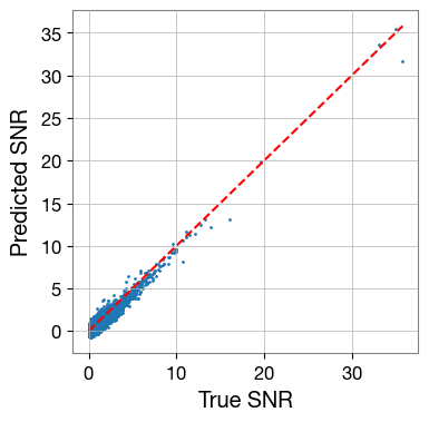
# predicted snr, using ANN model
pred_snr = gwsnr.optimal_snr_with_ann(gw_param_dict='./ler_data/IMRPhenomXPHM_O4_high_asd_L1_5.json')['L1']#['snr_net']

[27]:

from gwsnr.utils import get_param_from_json
true_snr = get_param_from_json('./ler_data/IMRPhenomXPHM_O4_high_asd_L1_5.json')['L1']#['snr_net']

[28]:

# select only snr between 4 and 12
# snr_min = 4
# snr_max = 12
# mask = (true_snr >= snr_min) & (true_snr <= snr_max)
# true_snr = true_snr[mask]
# pred_snr = pred_snr[mask]

# plot the predicted snr vs true snr
plt.figure(figsize=[4,4])
plt.scatter(true_snr, pred_snr, s=1)
snr_lim = [np.min([true_snr, true_snr]), np.max([true_snr, true_snr])]
plt.plot(snr_lim, snr_lim, 'r--')
plt.xlabel('True SNR')
plt.ylabel('Predicted SNR')
# plt.xlim([snr_min, snr_max])
# plt.ylim([snr_min, snr_max])
plt.show()

../_images/examples_model_generation_34_0.png

[29]:

# use the following function to predict the pdet
pred_pdet = np.array([1 if snr >= 8.0 else 0 for snr in pred_snr])
# true pdet
true_pdet = np.array([1 if snr >= 8.0 else 0 for snr in true_snr])

from sklearn.metrics import confusion_matrix, accuracy_score
cm = confusion_matrix(true_pdet, pred_pdet)
print(cm)

acc = accuracy_score(true_pdet, pred_pdet)
print(acc)

[[19966     0]
 [    7    27]]
0.99965

[ ]: